Tutorials > Jet Pump Design Basics

Introduction:

Many examples are provided in the samples datasets folder that use Jet-Pumps. However, it is assumed that the user is familiar with the concepts of hydraulic pumping, jet pump operation, and the size designations of jet pumps. If not, a short Jet-Pump Primer is presented here. If additional information is required, a useful jet pump reference is "JET PUMPING OIL WELLS." by Hal Petrie, Phil Wilson, and Eddie Smart. This is a series of three articles which appeared in WORLD OIL magazine in November 1983, December 1983, and January 1984. (NOTE: The equations presented in this series of articles are intended to be used with handheld calculators as opposed to computers.) Also recommended is Chapter 6 of the PETROLEUM ENGINEERING HANDBOOK published by the Society of Petroleum Engineers. This chapter on hydraulic pumping contains further information on jet pumps and contains the algorithms upon which the SNAP jet-pump design is based.

Jet Pump performance Theory:

The specific jet pump performance relationships used in SNAP are based on experimental performance curves incorporating nozzle and throat sizes using water tests. Since the Reynolds Number in the nozzle is always high, only specific gravity corrections are made when oil is used as a power fluid. The Reynolds Number in the throat however, varies widely depending on the production rate and viscosity. For this reason, a performance correction for produced fluid viscosity is included. This correction is based on jet pump testing done with Amoco Research on heavy oil with viscosities between 700 and 1900 cp.

Further performance corrections are made for density differences between the power fluid and produced fluid. This includes the effect of free gas on the average density of the produced fluid. Free gas is handled as additional liquid, with an appropriate gas interference correction factor. The same nozzle and throat. sizes may be used in a variety of pumps and bottom hole assemblies. No corrections are made to account for the different pressure drops that would exist in the various assemblies and configurations possible for installation. If the nozzle and throat size limits and flow limits shown in Trico Industries, Inc. specifications are adhered to, then no corrections have been found to be necessary. Most recently, improvements in high GOR modeling were implemented to correct errors in the TRICO 4.1 Jet pump program.

As with all SNAP models, well fluids are corrected for temperature and pressure. Specific gravity, viscosity, shrinkage, solubility and formation volume factors are calculated at the appropriate spot in the vertical profile of the well. A linear temperature gradient from the surface to the pump is assumed for the internal pump calculations. Steam vaporization is possible in high temperature, low pressure conditions but the steam will be modeled as a low density water phase and not as a gas.

Power fluid friction is calculated for the appropriate tubing size and fluid properties specified using descriptive data from all the panels. In the KOBE 4.1 Jet pump program, if gas is present, the return friction to the surface is calculated for the mix of power fluid and gassy produced fluid by means of the Orkiszewski Vertical Flowing Gradient Correlation. In SNAP, a full suite of hydraulics and produced fluid PVT relationships are available.

Jet pump cavitation limits are calculated for each pump intake pressure. The cavitation limit at a given pump intake pressure is the maximum flow possible. Operating at or very near this limit will also result in cavitation erosion of the throat and subsequent diminished pump performance. The cavitation relationship accounts for free gas by assuming choked flow, and corrects for temperature using values from steam tables for the

The performance of a jet nozzle and throat combination is related to the size of the nozzle and the annular area between the throat and the jet stream of the nozzle. The flow area of KOBE nozzles and throats increases as a geometric progression of 101/9. The flow area of any KOBE nozzle or throat is a constant multiple of 101/9 of the area of the next smaller size. The flow area of OILMASTER nozzles and throats increases as a geometric progression of 4/PI. The flow area of any OILMASTER nozzle or throat is a constant multiple 4/PI of the area of the next smaller size.

As the nozzle size and throat size increases, then the flow capacity increases. The larger nozzle flow area allows for greater nozzle flow and the larger annular area allows for larger volumes of oil, water, and gas to pass into the throat for the same differential pressure.

The ratio of the nozzle area to the throat area equals the area ratio. The program incorporates eight area ratios as follows: Y,X,A,B,C,D, E and F. The F ratio has the same area ratio as the E (throat 4 sizes larger than the nozzle) but with the World Oil curve instead of the KOBE curve.

Each nozzle and throat is assigned a size number based on the above geometric progression. A given nozzle size matched with the same numbered throat size will always give the same area ratio arid is designated as the A area ratio. The size designation 7-A is a size 7 nozzle in combination with a size 7 throat. Successively larger throats matched with a given nozzle size give the area ratios B, C, D, E, and F. A 7C is a size 7 nozzle with a size 9 throat. The area .ratio decreases; for each throat size greater than the nozzle. size number. The X and Y area ratios describe throat and nozzle combinations in which the throat size is less than the A ratio throat size for that nozzle size. The X and Y area ratio is larger than the A area ratio since the throat sizes are smaller.

As the area ratio progressively decreases from the A area ratio the throat size is increasing (B +1, C +2, D +3, E +4, and F +4). Area ratios with an increasing throat size have a greater annular area for the flow of fluid around the nozzle. Greater production rates are possible for a constant differential pressure, but less discharge head will develop due to shear effects that degrade the pressure recovery during mixing of the power fluid and the well produced fluids in the larger throats.

The reverse is true for the X and Y area ratios. Lower production rates occur as the throat size decreases (X -1, and Y -2) since the annular area available for fluid flow is progressively decreasing. Greater discharge head will develop due to better pressure recovery resulting from a reduction in the shear effects occurring in the smaller throats.

Design hints and workflow (based on the Trico Jet-Pump Manual):

In many cases you will be trying to select an optimum size within a horsepower constraint. The power required depends on the nozzle size, the operating pressure, the depth of the well, and the pump intake pressure. By trying a couple of sizes one can quickly determine the largest nozzle size that will match the horsepower limit. For a given nozzle size, there will be an optimum throat size (area ratio) to maximize production at a given power fluid pressure and pump intake pressure. By trying different ratios with the same nozzle size, the optimum ratio can be determined.

In general, larger throats with. a given nozzle lead to higher operating pressures because these ratios have. less pressure recovery. However, when power fluid friction is significant, the use of a larger ratio may lead to lower operating pressure if the nozzle size can also be reduced. To maximize the efficiency of a jet pump system use the smallest nozzle possible that prevents cavitation while operating at the highest power fluid pressure. The object is to minimize the power fluid loading while using the most efficient nozzle and throat combination. For example, an 8B use the same throat as a 9A, but has a larger annular area for cavitation and will use less power fluid at the same operating pressure. Normally the B ratio would require a higher operating pressure, but the savings in power fluid and return friction pressure drop may offset this. The only way to tell is to run several sizes and see which is the most efficient and which matches the surface power unit best. The system designed must also minimize the amount of power fluid that is bypassed by the pressure controller on the surface equipment since this is a direct waste of energy.

Related to the above discussion is the effect of pump discharge pressure on pump performance. Generally, it takes from 3 to 5 extra psi of power fluid pressure to maintain performance if the discharge pressure is increased by 1 psi. This depends on the ratio, with the higher ratios being more sensitive. The discharge pressure depends on the gas-to-liquid ratio (GLR) in the return column. The return GLR depends on how much power fluid is mixed with the production. The use of a smaller nozzle can increase the GLR, lower the pump discharge pressure, and allow the use of a larger ratio pump in some cases.

In wells deeper than about 6000 feet, the use of oil power fluid typically results in better performance due to the decreased hydrostatic head. Although the use of water as a power fluid increases the pressure at the nozzle, due to its higher density, it also increases the discharge pressure. This latter effect dominates and becomes evident in deeper wells. A power water system, when used in deep wells, tends to “load up” the return column and stalls out the jet pump because of the high discharge pressure required to lift the water.

In vertical multi-phase flow, there is an optimum pipe or annulus size that will give a minimum pump discharge pressure. In the absence of gas, bigger is better on the return path, but with gas this may not be true due to changes in the type of flow regime that occur. By comparing casing and tubing returns (casing free versus parallel installations) you can see the effect of return conduit size.

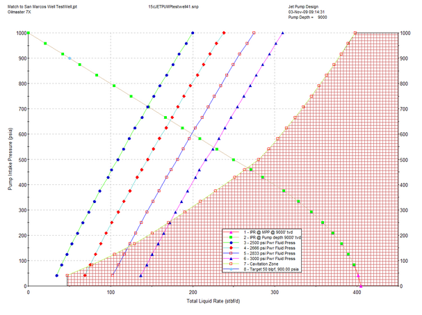
Remember that the program calculates a matrix of possible jet pump operating points for the well completion described by the input data. The actual performance is the intersection of the well performance (IPR) curve with pump performance curves for the power fluid pressures selected. Therefore, on a given plot of pump performance, any number of well performance curves can be drawn and the appropriate intersections noted.

Sample Jet Pump Output plot:

Sample JetPump Output report:

----------------------------------------------------------------------------------- Page 1

SNAP Jet Pump Module Running With Snap 2.143.497 10/14/2009

Developed By Ryder Scott Company with funding from ConocoPhillips Alaska, Inc. 2005

Solution Algorithm based on SPE Petroleum Engineering Handbook, Hal Petrie, 1990

Original pump performance relationship copyright Weatherford, Hai Phan 1982

--------------------------------------------------------------------------------------------

Dataset: 15cJETPUMPtestwell41.snp

Title: Match to San Marcos Well TestWell.jpt

----------------------------------------------------------------------------------------------

1) Perforation Depth (ft) : 9000 13) Producing GOR (scf/STB) : 100

2) Pump Vertical Depth (ft) : 9000 14) Gas Sp. Gravity (air=1.) : 0.850

3) Pump Installation 15) Separator Press (psig) : 100.0

Casing installation 16) Well Static BHP (psig) : 1000.0

4) Casing (production) ID (in) : 4.892 17) Pump Intake Press (psig) : 900.0

5) N/A 18) Well Test Flow Rate(bpd) : 50.0

6) Power Tubing ID (in) : 2.441 19) Well Head Temp (deg F) : 100.0

7) Power Tubing OD (in) : 2.875 20) Bottom Hole Temp (deg F) : 205.0

8) Tubing Length (ft) : 9100 21) Not Vented : Not Vented

9) Pipe Roughness e/d (in/in) : 0.0018 22) Power Fluid oil/water : Oil

10) Oil Gravity (API) : 30.000 23) Power Fluid API : 30.03

11) Produced Vol Water Cut (%) : 19.60 24) Bubble Point Press(psig) : N/A

12) Water Specific Gravity : 1.030 25) Well Head Press (psig) : 100.0

=======================================================================================

Oilmaster 7X Pump Performance Summary

Target Production Rate of 50 BLPD at 900 psig pump intake pressure

Predicted Surface Power Fluid Injection Pressure at Target = 1924 psig

Predicted Surface Power Fluid Injection Rate at Target = 948 bpf/d

Predicted Pump Intake Pressure at Target = 900 psig

Predicted Pump Discharge Pressure at Target = 3367 psig

Predicted Power Fluid Pressure at Pump depth at Target = 5247 psig

=======================================================================================

----------------- ----------------- ----------------- -----------------

Match Prod Rate (blpd) Rate= 145 Rate= 173 Rate= 199 Rate= 226

Match Pwr Fluid Press (psig) PFP = 2500 PFP = 2666 PFP = 2833 PFP = 3000

Match Pwr Fluid Rate (blpd) QN = 1023 QN = 1044 QN = 1065 QN = 1086

Match Pump Intake Pres(psig) PIP = 709 PIP = 654 PIP = 602 PIP = 548

Pump Discharge Prs(psig) PD = 3375 PD = 3378 PD = 3382 PD = 3382

Match Pwr Fld prs @pmp (psig) PN = 5832 PN = 6000 PN = 6170 PN = 6339

----------------- ----------------- ----------------- -----------------

PmpInPr Qresvr QCav QSuctn QNozzl cd QSuctn QNozzl cd QSuctn QNozzl cd QSuctn QNozzl cd

PSIG STB/D STB/D STB/D B/D STB/D B/D STB/D B/D STB/D B/D

------ ------- ------- ------- ------- - ------- ------- - ------- ------- - ------- ------- -

1000 0 398 200 993 0 238 1010 0 274 1027 0 309 1043 0

958 21 389 192 998 0 229 1014 0 266 1031 0 301 1047 0

917 42 381 183 1002 0 221 1018 0 257 1035 0 293 1051 0

875 63 372 176 1006 0 213 1023 0 249 1039 0 285 1055 0

833 83 363 168 1010 0 206 1027 0 242 1043 0 278 1059 0

792 104 354 160 1014 0 197 1031 0 234 1047 0 270 1063 0

750 125 344 152 1019 0 189 1035 0 226 1051 0 262 1067 0

708 146 335 145 1023 0 182 1039 0 219 1055 0 254 1071 0

667 167 325 138 1027 0 175 1043 0 212 1059 0 247 1075 0

625 188 314 130 1031 0 168 1047 0 203 1063 0 239 1079 0

583 208 304 123 1035 0 159 1051 0 196 1067 0 232 1083 0

542 229 293 116 1039 0 152 1055 0 188 1071 0 224 1087 0

500 250 280 109 1043 0 145 1059 0 181 1075 0 216 1091 0

458 271 263 101 1047 0 138 1063 0 173 1079 0 208 1095 0

429 285 251 97 1050 0 132 1066 0 168 1082 0 203 1097 0

375 311 228 87 1056 0 123 1071 0 159 1087 0 194 1102 0

333 329 209 80 1060 0 116 1075 0 152 1091 0 187 1106 0

292 344 190 74 1064 0 109 1079 0 144 1095 0 179 1110 0

250 358 171 66 1068 0 102 1083 0 137 1099 0 172 1114 0

208 371 151 60 1072 0 95 1087 0 130 1102 0 165 1118 0

167 381 129 53 1076 0 88 1091 0 124 1106 0 158 1121 0

125 390 105 47 1079 0 82 1095 0 117 1110 0 151 1125 0

83 396 77 40 1083 0 75 1099 0 110 1114 0 144 1129 4

42 401 47 34 1087 0 69 1103 0 102 1118 0 137 1133 4

1 405 0 27 1091 0 62 1106 0 96 1121 0 130 1136 0

---------------------- ----------------- ----------------- ----------------- -----------------

Maximum HP Required HP = 53 HP = 58 HP = 62 HP = 67

Successful Codes (cd): 0 = normal JP operation, 1 = Well flowing, 2 = Pump stalling

Failure Codes : 3 = could not find operating point, 4 Function diverges from solution:min error given

=======================================================================================

----------------------------------------------------------------------------------- Page 2

SNAP Jet Pump Module Running With Snap 2.143.497 10/14/2009

Developed By Ryder Scott Company with funding from ConocoPhillips Alaska, Inc. 2005

Solution Algorithm based on SPE Petroleum Engineering Handbook, Hal Petrie, 1990

--------------------------------------------------------------------------------------------

Dataset: 15cJETPUMPtestwell41.snp

Title: Match to San Marcos Well TestWell.jpt

----------------------------------------------------------------------------------------------

Detailed Iteration Results for Solution Point Page 2

This single page report attempts to re-run the jet-pump calculations at the predicted

Solution point from the prior calculations. If this point solves back to the Target

Rate and pressure, it indicates that the solution is of high quality. Conversly, if the

last QLS value in the following table if far different from the target, a poor

solution is indicated.

Single Point Iteration Results for Solution Conditions

Target Production Rate of 50 BLPD at 900 psig pump intake pressure

Predicted Surface Power Fluid Injection Pressure at Target = 1924 psig

Predicted Surface Power Fluid Injection Rate at Target = 948 bpf/d

Predicted Pump Intake Pressure at Target = 900 psig

ANOZ= 0.0104 in2 AANN= 0.0110 in2 SPGPF= 0.8760 VISPF= 4.0973 cp NzPrs= 5247.1 psig

SPGO= 0.8002 FVFO= 1.1163 SPGW= 1.0300 FVFW= 1.0436 SPGS= 0.8368

QN= 948 PLN= 4 QCAV= 377 HP= 36 hp FVPFU= 1.0269

GOR= 100 GORS= 100 FREEGOR= 0 FVFG= 0.0184 DENAVE= 0.0000

Pwr Fluid Flow Area ID= 2.441 Equv Rad ID= 2.44 dpfric= 4.1 Nrey= 2330.48

Iter QS QOSTB DQS QD PrsDis CMR FX PR DENR QLS Error% QGS Code

0 1263.13 922 157.77 2211 3401 1.3337 -0.5915100 0.5753 0.980 1263 2426.3% 0 3

1 1263.13 922 157.77 2211 3401 1.3337 -0.5920176 0.5753 0.983 1263 2426.3% 0 3

2 1105.36 806 157.77 2053 3397 1.1671 -0.5010337 0.5744 0.981 1105 2110.7% 0 3

3 947.60 691 157.77 1895 3407 1.0005 -0.4211380 0.5767 0.981 948 1795.2% 0 3

4 116.00 85 78.88 1064 3371 0.1225 -0.0330463 0.5683 0.981 116 132.0% 0 3

5 45.19 33 39.44 993 3364 0.0477 0.0016319 0.5668 0.981 45 -9.6% 0 3

6 48.52 35 1.00 996 3363 0.0512 0.0002775 0.5666 0.981 49 -3.0% 0 0