|
<< Click to Display Table of Contents >> General Tutorial |
  
|
|
<< Click to Display Table of Contents >> General Tutorial |
|
The SNAP tutorial gives step-by-step instructions for creating a SNAP project. The tour uses the SNAP Default Dataset.SNP file, which is included with your SNAP application. Working through the SNAP tutorial is an excellent way to become proficient with SNAP.
Beginning the Snap Tutorial
We will begin by starting SNAP. If you have not yet installed SNAP, please take the time to do so.
| 1. | Double-click the SNAP icon or in Windows, from the taskbar choose Start>> Programs>> SNAP in order to open the program. |

| 2. | Choose File>> Open Dataset. The Open Dataset dialog box appears. |
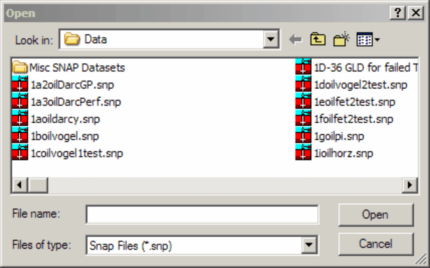
| 3. | In the Open Dataset dialog box, select SNAP Default Dataset.SNP. |
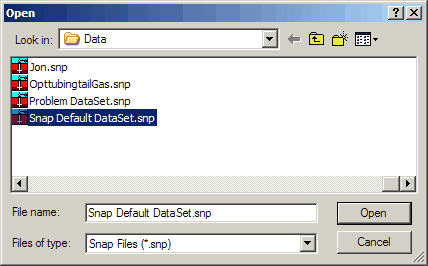 |
| After selecting the file, click Open. |
General Project Definition
In SNAP, you begin defining the well system in the General Project Definition dialog box. Gain access to this dialog box by clicking the General button on the schematic
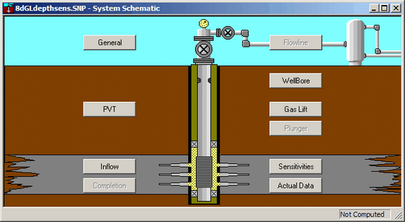
or by selecting General from the toolbar using this button -> ![]()
You will see this screen:
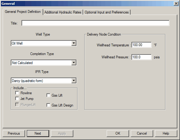
In this dialog box, you can name your dataset, indicate whether the primary phase is oil or gas, and select an IPR type to define system temperatures and pressures, as well as other system conditions.
Well Type
SNAP performs calculations on the following well types:
| • | Oil Well |
| • | Gas Well |
| • | Water Injector |
| • | Gas Injector |
Completion Type
The Completion Type is dependent upon the IPR chosen for evaluation.
Completion Type options are:
| • | Not Calculated |
| • | Cased/Gravel Packed |
| • | Perforated |
IPR Type
Online Help explains each IPR Type in the Inflow Reservoir and Well Data sections. The IPR equations in SNAP include:
| • | Darcy's Law |
| • | Vogel's Method with Reservoir Data |
| • | Vogel's from One Rate Test |
| • | Vogel's from Two Rate Test |
| • | Fetkovich from Multipoint Test |
| • | Conventional Flow-After-Flow Test |
| • | Isochronal Test |
| • | Modified Isochronal Test |
| • | Fetkovich from C and N |
| • | Constant Productivity Index |
| • | Babu & Odeh Horizontal Well Model |
| • | Fractured Well Model |
| • | Quadratic Flow Equation |
| • | Back Pressure C and N |
General Project Definition Exercise
The following steps will demonstrate how the selections you make in the General Project Definition dialog box affect the end results.
| 1. | Click General on the SNAP schematic to open the General Project Definition dialog box. |
| 2. | For IPR Type, Select Vogel's Method with Reservoir Data. |
Note: Making changes early on may activate or remove certain input panels. It is a good idea to make sure you have data in the correct locations and are not left with empty dialogs that were not previously available.
| 3. | Click the Optional Hydraulic Rates tab. The Optional Hydraulic Rates dialog box opens. This is used to enter flow rates of interest, which appear as symbols on the IPR curve(s). |
| Enter the following flow rates: |
#1 |
1200 |
#2 |
1400 |
#3 |
1600 |
#4 |
1800 |
#5 |
2000 |
and click OK.
| 4. | Return to the General Project Definition window by clicking General again. Click the Next button to proceed to the PVT dialog box. |
| (You can also access the PVT dialog box by clicking the PVT Button on the toolbar |
PVT Properties
The PVT Properties dialog box enables you to enter basic reservoir pressure, volume, and temperature data (hence the name "PVT") to describe a reservoir's fluid. PVT parameters are pressure dependent and therefore change with time.
This dialog box changes slightly depending on whether you select an oil well or a gas well. For an oil well, specific correlations are available for determining the gas/oil ratio (GOR), formation volume factor (Bo), and oil viscosity. The differences in the oil correlations represent the variances in the type of reservoir fluid or oil properties. Help>>Input Panels>>PVT Properties gives information about which correlation is appropriate to use under specific circumstances.
If you select a gas well, there are no correlations available and SNAP deactivates the Oil API Gravity and Water Specific Gravity fields.
PVT Exercise
| 1. | The PVT window should be displayed from where we left off. (If not, click the PVT Button from the toolbar. |
| 2. | View the available correlations on the drop down lists for Solution Gas/ Oil Ratio, Oil Formation Volume, and Oil Viscosity. Leave the original selections. |
| 3. | Click Next to proceed to the Inflow Properties dialog box. |
Inflow Properties
The Inflow dialog box is specific to the type of IPR you select in the General Projection Definition dialog box. The IPR type selected for the tour is Vogel's Method with Fluid Data, therefore choosing the Inflow command displays the corresponding dialog box. Use this dialog box to enter data for the various single- and multi-point correlations that SNAP uses in pressure drop calculations.
This page can be accessed through the Inflow button on the toolbar![]() , by clicking the Inflow button on the schematic, or choosing Inputs>> Inflow to open the Constant PI from Fluid Levels dialog box.
, by clicking the Inflow button on the schematic, or choosing Inputs>> Inflow to open the Constant PI from Fluid Levels dialog box.
Inflow Properties Exercise
| 1. | Start with the dialog box |
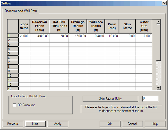
| 2. | Change the Reservoir Pressure to 3000 psi. |
| 3. | Click the Next button to proceed to the Flowline Geometry dialog box. (If you reach the Wellbore page, go back to General and check the Include>> Flowline option box. Then click Flowline on the schematic.) |
Completion Data
The Completion Data dialog box is not active because the IPR equation selected for this tutorial does not require Completion Type user input to perform necessary calculations. When the dialog box is active, you can fine tune the completion algorithms for the corresponding equations. You can model up to five commingled zones when using Darcy's Law or Vogel's Method with reservoir data.
Flowline Geometry
The total length of the flowline is described using pipe diameter changes, non-linear temperature profiles, and segments that describe the flowline profile. You begin describing the geometry at the separator and work towards the wellhead. Because the flowline components' elevations affect performance relationships, SNAP offers three methods for calculating flowline geometry. These methods are ML (Measured Length) versus Angle, ML versus Elevation, and Elevation versus Angle or click the Flowline button on the toolbar.
You can choose from the following five hydraulic correlations:
| · | Dukler |
| · | Beggs & Brill |
| · | Mukherjee & Brill |
| · | Dukler& Eaton |
| · | Minami-Beggs-Brill |
Flowline Geometry Exercise
| 1. | If the Flowline Geometry dialog box is not displayed, select Flowline from the toolbar to open this dialog box |
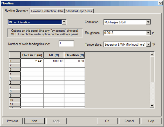
| 2. | In the Flow Line ID (in) column, click the 2.441 data value. |
| 3. | Next click the Standard Pipe Sizes tab to open the Dimensions of Standard Tubing dialog box. |
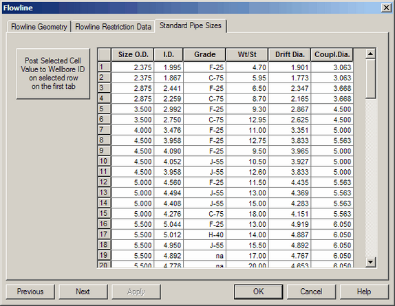
| 4. | Locate and click the row that has the tubing dimensions with an ID (inside diameter) of 1.995 for P-110 Grade. |
| 5. | Click the OK button to return to the Flowline Geometry dialog box. Notice that the flowline ID dimension has been automatically updated. |
Wellbore Geometry
Wellbore Geometry can be a single tubing string or multiple strings depicted as individual segments that describe the wellbore. You begin at the wellhead and end at the bottom of the hole. You can also model either annular or tubular flow. Hydraulic correlations include: Hagedorn and Brown, Orkiszewski, Duns and Ros, Aziz, Beggs and Brill, Gray, Mona, Modified Gray, Dus-Ros-Gray, Mechanistic, and Cullender-Smith. Click Hydraulics Correlation to open the Correlation advisor.
Wellbore Geometry Exercise
| 1. | If the Wellbore Geometry dialog box is not displayed, select Wellbore from the toolbar. Optionally, if the schematic is displayed, click the Wellbore button. |
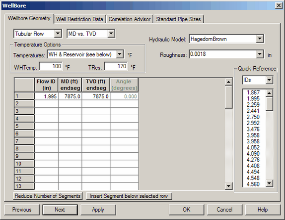
| 2. | Click the Correlation Advisor button to open the Correlation Advisor dialog box. |
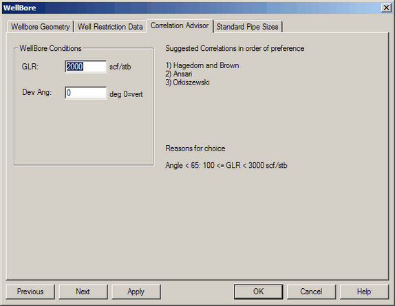
| 3. | Click the Update button. In the Suggested Correlations section, the Correlation Advisor suggests the best correlations to use based on the data input. Observe this information to decide which works best for the current analysis. When you return to the Wellbore Geometry dialog box, you can select one of these options. |
| 4. | Click the Done button to exit this dialog box. |
| 5. | Click the Next button to proceed to the Sensitivities dialog box. |
Gas Lift
If your well uses gas lift, you need to provide SNAP with gas lift characteristics to obtain an accurate analysis. SNAP only enables the Gas Lift item if you select the Include Gas Lift check box in the General Project Definition dialog box.
Note: For this tour, Gas Lift is not being considered, and therefore, the option was not activated in the General Project Definition dialog box.
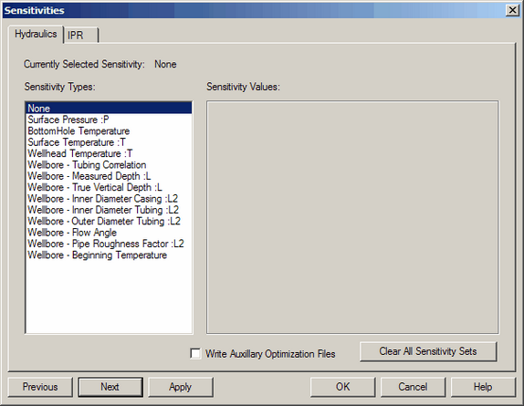
Sensitivities for Calculations
| You can use the SNAP Sensitivities dialog box to vary system parameters and evaluate their overall effects on IPR and hydraulics. SNAP displays each effect as an additional curve on the results graph when you run calculations. SNAP does not list selections that are not applicable (such as Flowline ID when no flowline is defined) as available sensitivities. You have the option to enter Tubing, Reservoir, or Combined sensitivities. |
| Sensitivities Exercise |
| 1. | If the Sensitivities dialog box is not already displayed, click the sensitivities button on the toolbar. |
| 2. | Change the flowline pressures to correspond with the following: |
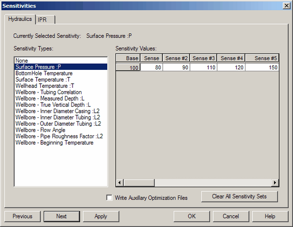
| 3. | Click the OK button to save the changes and return to the Sensitivities dialog box. |
| 4. | Click the X button to close the Sensitivities dialog box. |
Calculating the Nodal System
| After entering all the data, you proceed to calculate the nodal analysis. Here you have the option of calculating the entire analysis, just the IPR curve set, or just the hydraulic curves. |
| Calculation Exercise |
| 1. | Choose Calculate>>Calculate All to calculate both the IPR curves and the hydraulic curves. |
| 2. | View the plot that is displayed after the calculation is complete. Notice each of the sensitivity curves for IPR and hydraulics as well as the symbol locations of the Optional Hydraulic Flowrates, Minimum Lift Rate, and Minimum Flow Rate. |
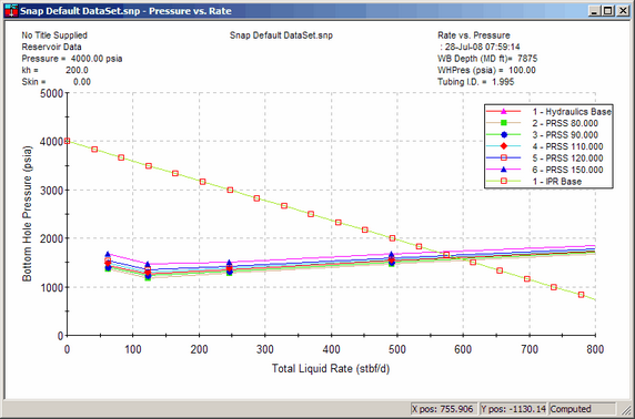
Plots
After entering and editing data in the options dialog boxes, you can generate, manipulate, and print IPR, hydraulics, and system plots. You can also elect to generate a gradient plot of the baseline and optional hydraulic flowrates. See “Calculate Menu” on page 71 for further information on this topic.
When you generate a plot using Calculate, it is displayed in a Plot Viewer window. As a Result, tree new menu items appear on the menu bar, the new menu items are:
| • | Edit- enables customization of plot layout, color, fonts and other characteristics for printing. |
| • | Tools- enables zoom in and out of regions on the plot and view a project summary. |
| • | Plots- enable viewing of graphical representations of the calculated values. |
SNAP can generate any of the following five types of plots:
| • | Rate vs. Reservoir Pressure |
| • | BH Pressure vs. Reservoir Pressure |
| • | Rate vs. Flowline Pressure |
| • | BH Pressure vs. Flowline Pressure |
| • | Gradient Curve |
Plots Exercise
To view the generated plots:
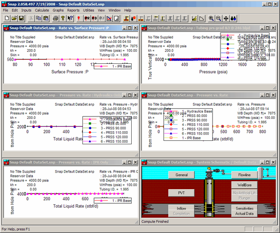
| 1. | Choose Graphs>> Sensitivity Results>> Rate vs. Surface Pressure from the menu. The Surface Pressure plot appears. |
| 2. | Proceed to open the next four plots as in step 1. Each plot opens in the SNAP application window. |
| 3. | Now choose Window>> Tile to view all the plots as shown in the following illustration. |
Report Format
Although you can display and print results graphically in SNAP, you may also find it necessary to obtain results in report format. SNAP automatically generates reports after you have performed a calculation on the system.
Report Exercise
| 1. | Choose Reports>> Summary to display a summary report. Or to display a gradient report choose Reports>> Gradient. |
| 2. | After viewing the report, close the window. |
To Exit SNAP
To exit SNAP choose File>> Exit.